Joint Frequency Table

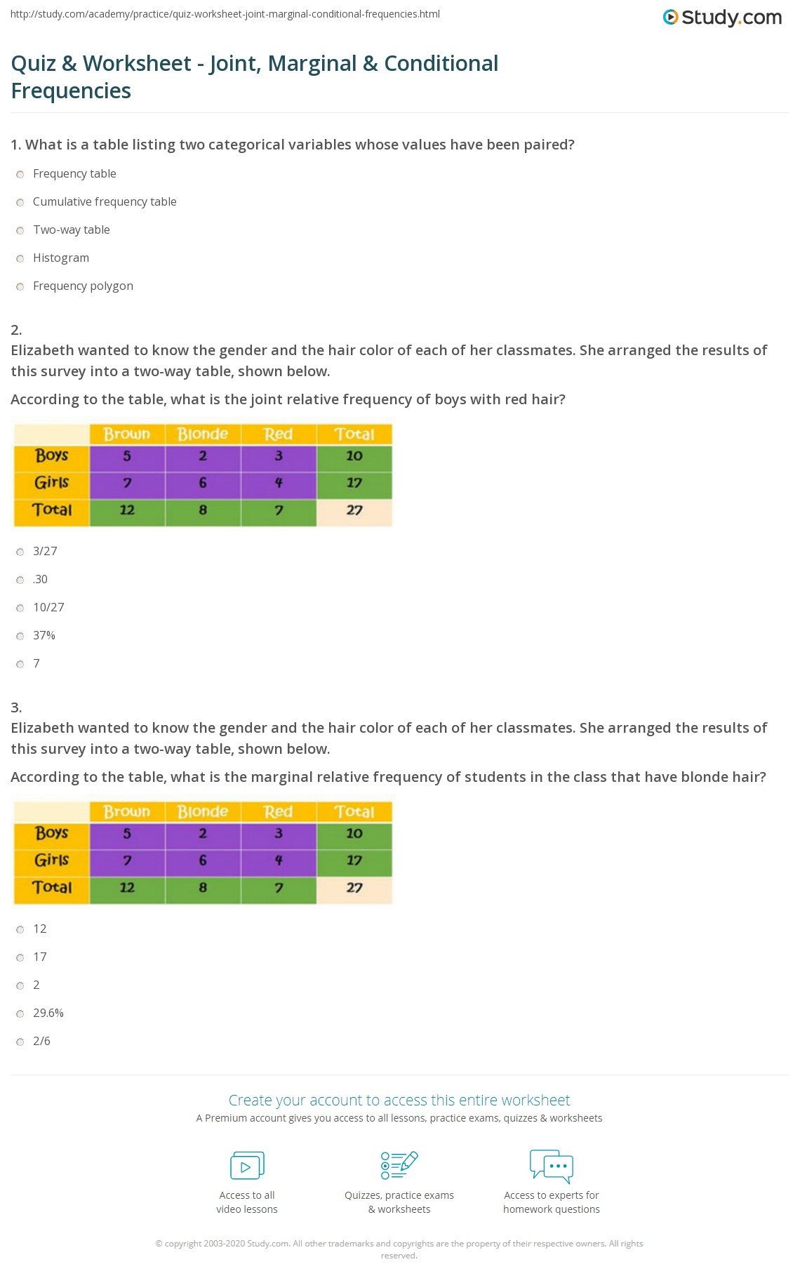
When analyzing relationships between two categorical variables, I’ve often found myself reaching for a joint frequency table. It’s a simple yet powerful tool that lays out the co-occurrence of categories in a clear, structured format. For example, if you’re studying the relationship between smoking habits and lung health, a joint frequency table can show you exactly how many non-smokers have healthy lungs versus how many smokers don’t. The beauty of this tool is its ability to condense complex data into a digestible format, making it easier to spot patterns or dependencies.

Table of Contents

What is a Joint Frequency Table?

A joint frequency table is essentially a grid that displays the frequency of each combination of categories from two variables. Think of it as a spreadsheet where rows represent one variable and columns represent the other. Each cell in the table contains the count (or frequency) of observations that fall into both categories simultaneously. For instance, if you’re analyzing survey data on preferred coffee types and age groups, the table would show how many 20-somethings prefer lattes versus how many 50-somethings opt for black coffee.

Here’s the thing: while it sounds straightforward, the value of a joint frequency table lies in its ability to reveal associations that might not be obvious from raw data. It’s not just about counting; it’s about understanding how variables interact. In my experience, this tool is particularly useful in exploratory data analysis, where you’re trying to uncover hidden relationships before diving into more complex statistical tests.

How to Create a Joint Frequency Table

Creating a joint frequency table is simpler than it might seem, especially with the right tools. Here’s a step-by-step guide based on my hands-on experience:

Identify Your Variables: Start by selecting the two categorical variables you want to analyze. Ensure they’re both discrete and have a manageable number of categories.
Collect Your Data: Gather the dataset containing observations for both variables. This could be survey responses, experimental results, or any other source of categorical data.
Organize the Table: Set up a grid where one variable forms the rows and the other forms the columns. Label each row and column clearly.
Count the Frequencies: For each combination of categories, count how many observations fall into that pair. Fill these counts into the corresponding cells of the table.
Add Marginal Totals: Include row and column totals to show the overall frequency of each category. This helps in understanding the distribution of each variable independently.

📊 Note: When working with large datasets, consider using software like Excel, Python’s pandas, or R to automate the process. Manually counting frequencies can be error-prone and time-consuming.

Interpreting a Joint Frequency Table

Once your joint frequency table is ready, the real work begins: interpretation. Here’s how I approach it:

Look for Patterns: Are certain combinations more frequent than others? For example, do younger people tend to prefer certain products over older individuals?
Compare Marginal Totals: Do the row or column totals reveal any imbalances? This can indicate differences in the distribution of one variable across categories of the other.
Calculate Conditional Frequencies: Divide the cell frequencies by the row or column totals to understand the proportion of one category given the other. This helps in identifying dependencies.

Honestly, the most insightful moments come when you compare expected frequencies (based on independence) with observed frequencies. If they differ significantly, it suggests a relationship between the variables. This is where the joint frequency table truly shines—it sets the stage for more advanced analyses like chi-square tests.

Common Pitfalls to Avoid

While joint frequency tables are incredibly useful, there are a few pitfalls I’ve encountered that are worth mentioning:

Overlooking Small Sample Sizes: If certain cells have very low frequencies, it can skew interpretations. Always consider the sample size before drawing conclusions.
Assuming Causation: A joint frequency table shows associations, not causation. Don’t jump to conclusions about one variable causing changes in another without further evidence.
Ignoring Marginal Totals: Failing to include row and column totals can lead to incomplete analysis. These totals provide crucial context for understanding each variable’s distribution.

⚠️ Note: Always cross-check your findings with other analytical methods to ensure robustness. A joint frequency table is just one piece of the puzzle.

Practical Applications

In my experience, joint frequency tables are versatile tools applicable across various fields. Here are a few examples:

Marketing: Analyzing customer preferences by demographics to tailor campaigns.
Healthcare: Studying the relationship between lifestyle choices and health outcomes.
Social Sciences: Examining voting patterns across different age groups or regions.

That said, the key is to match the tool to the question you’re trying to answer. Not every research question requires a joint frequency table, but when it does, it’s invaluable.

A joint frequency table is more than just a grid of numbers—it’s a window into the relationships between variables. By mastering its creation and interpretation, you can uncover insights that might otherwise remain hidden. Remember, the goal isn’t just to count frequencies but to tell a story with your data. So, the next time you’re faced with categorical variables, give this tool a try. You might be surprised by what you discover.

Related Terms: